Published: 15.12.2022

PPO — Intuitive guide to state-of-the-art Reinforcement Learning

Introduction

Proximal Policy Optimization (PPO) has been a state-of-the-art Reinforcement Learning (RL) algorithm since its proposal in the paper Proximal Policy Optimization Algorithms (Schulman et. al., 2017). This elegant algorithm can be and has been used for various tasks. Recently, it has also been used in the training of ChatGPT, the hottest machine-learning model at the moment.

PPO is not just widely used within the RL community, but it is also an excellent introduction to tackling RL through Deep Learning (DL) models.

In this article, I give a quick overview of the field of Reinforcement Learning, the taxonomy of algorithms to solve RL problems, and a review of the PPO algorithm proposed in the paper. Finally, I share my own implementation of the PPO algorithm in PyTorch, comment on the obtained results and finish with a conclusion.

Reinforcement Learning

The classical picture that is first shown to people approaching RL is the following:

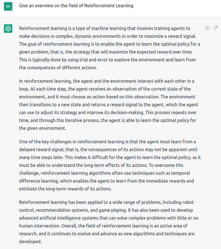
ChatGPT’s answer to the prompt: “Give an overview on the field of Reinforcement Learning”. While I asked help to ChatGPT for the introduction to the field of RL which was used to train ChatGPT itself (quite meta), I promise that everything in this article apart from this picture is written by me.

The classical picture that is first shown to people approaching RL is the following:

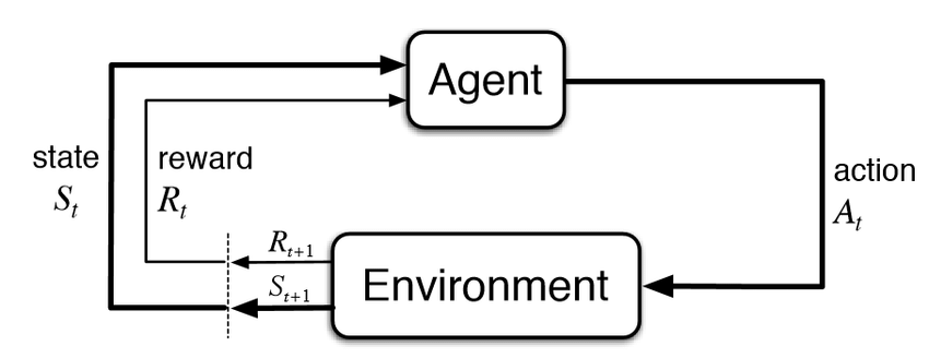
Reinforcement Learning framework. Image from neptune.ai

At each timestamp, the environment provides the agent with a reward and an observation of the current state. Given this information, the agent takes an action in the environment which responds with a new reward and state and so on. This very general framework can be applied in a variety of domains.

Our goal is to create an agent that can maximize the obtained rewards. In particular, we are typically interested in maximizing the sum of discounted rewards

Where γ is a discount factor typically in the range [0.95, 0.99], and r_t is the reward for timestamp t.

Algorithms

So how do we solve an RL problem? There are multiple algorithms, but they can be divided (for Markov Decision Processes or MDPs) into two categories: model-based (create a model of the environment) and model-free (just learn what to do given a state).

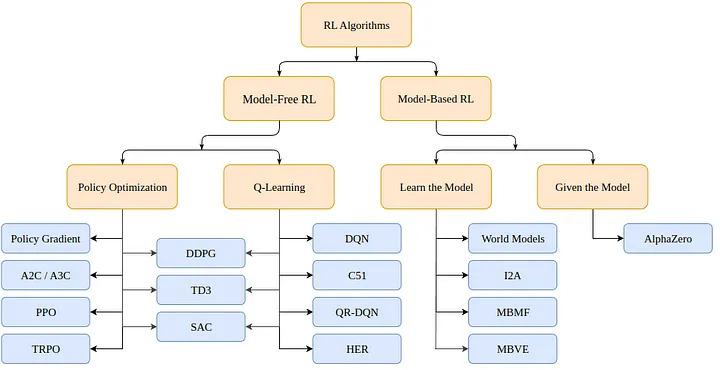
Taxonomy of Reinforcement Learning algorithms (from OpenAI spinning up)

Model-based algorithms use a model of the environment and use this model to predict future states and rewards. The model is either given (e.g. a chessboard) or learned.

Model-free algorithms instead, directly learn how to act for the states encountered during training (Policy Optimization or PO), which state-action pairs yield good rewards (Q-Learning), or both at the same time.

PPO falls in the PO family of algorithms. We do not thus need a model of the environment to learn with the PPO algorithm. The main difference between PO and Q-Learning algorithms is that PO algorithms can be used in environments with continuous action space (i.e. where our actions have real values) and can find the optimal policy even if that policy is a stochastic one (i.e. acts probabilistically), whereas the Q-Learning algorithms cannot do either of those things. That’s one more reason to prefer PO algorithms. On the other hand, Q-Learning algorithms tend to be simpler, more intuitive, and nicer to train.

Policy Optimization (Gradient-Based)

PO algorithms try to learn a policy directly. To do so, they either use gradient-free (e.g. genetic algorithms) or, perhaps more commonly, gradient-based algorithms.

By gradient-based methods, we refer to all methods that try to estimate the gradient of the learned policy with respect to the cumulative rewards. If we know this gradient (or an approximation of it), we can simply move the parameters of the policy toward the direction of the gradient to maximize rewards.

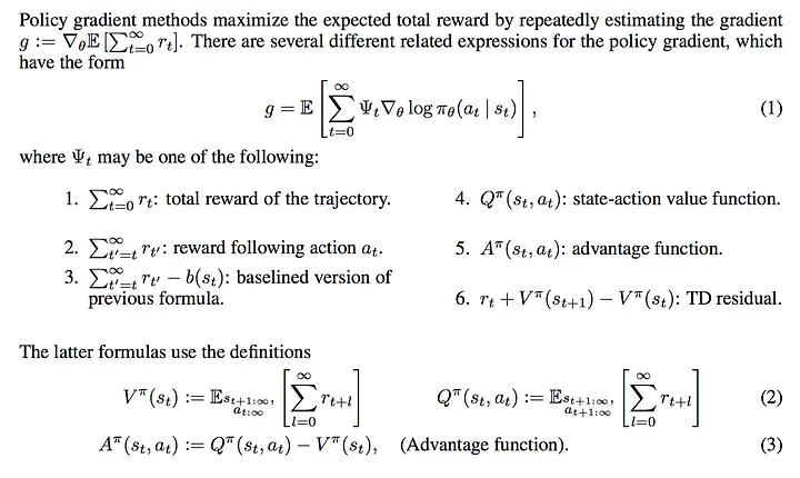
Objective to be maximized with PO algorithms. Image from Lil’Log’s blog.

Notice that there are multiple ways to estimate the gradient. Here we find listed 6 different values that we could pick as our maximization objective: the total reward, the reward following one action, the reward minus a baseline version, the state-action value function, the advantage function (used in the original PPO paper) and the temporal difference (TD) residual. In principle, they all provide an estimate of the real gradient we are interested in.

PPO

PPO is a (model-free) Policy Optimization Gradient-based algorithm. The algorithm aims to learn a policy that maximizes the obtained cumulative rewards given the experience during training.

It is composed of an actor πθ(. | st) which outputs a probability distribution for the next action given the state at timestamp t, and by a critic V(st) which estimates the expected cumulative reward from that state (a scalar). Since both actor and critic take the state as an input, a backbone architecture can be shared between the two networks which extract high-level features.

PPO aims at making the policy more likely to select actions that have a high “advantage”, that is, that have a much higher measured cumulative reward than what the critic could predict. At the same time, we do not wish to update the policy too much in a single step, as it will probably incur in optimization problems. Finally, we would like to provide a bonus for the policy if it has high entropy, as to motivate exploration over exploitation.

The total loss function (to be maximized) is composed of three terms: a CLIP term, a Value Function (VF) term, and an entropy bonus.

The final objective is the following:

The loss function of PPO to be maximized.

Where c1 and c2 are hyper-parameters that weigh the importance of the accuracy of the critic and exploration capabilities of the policy respectively.

CLIP Term

The loss function motivates, as we said, the maximization of the probability of actions that resulted in an advantage (or minimization of the probability if the actions resulted in a negative advantage):

First loss term. We maximize the expected advantage while not moving the policy too much.

Where:

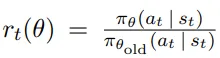
Coefficient rt(θ). This is the term that gradients are going to go through.

Is a ratio that measures how likely we are to do that previous action now (with an updated policy) with respect to before. In principle, we do not wish this coefficient to be too high, as it means that the policy changed abruptly. That’s why we take the minimum of it and the clipped version between [1-ϵ, 1+ϵ], where ϵ is a hyper-parameter.

The advantage is computed as:

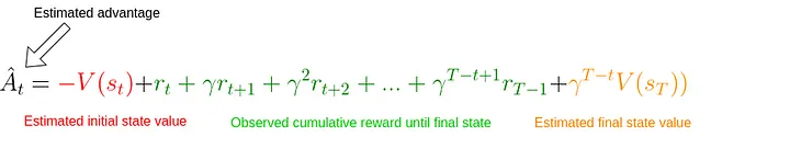
Advantage estimate. We simply take a difference between what we estimated the cumulative reward would have been given the initial state and the real cumulative reward observed up to a step t plus the estimate from that state onward. We apply a stop-gradient operator to this term in the CLIP loss.

We see that it simply measures how wrong the critic was for the given state st. If we obtained a higher cumulative reward, the advantage estimate will be positive and we will make the action we took in this state more likely. Vice-versa, if we expected a higher reward and we got a smaller one, the advantage estimate will be negative and we will make the action taken in this step less likely.

Notice that if we go all the way down to a state sT that was terminal, we do not need to rely on the critic itself and we can simply compare the critic with the actual cumulative reward. In that case, the estimate of the advantage is the true advantage. This is what we are going to do in our implementation of the cart-pole problem.

Value Function term

To have a good estimate of the advantage, however, we need a critic that can predict the value of a given state. This model is learned in a supervised fashion with a simple MSE loss:

The loss function for our critic is simply the Mean-Squared-Error between its predicted expected reward and the observed cumulative reward. We apply a stop-gradient operator only to the observed reward in this case and optimize the critic.

At each iteration, we update the critic too such that it will give us more and more accurate values for states as training progresses.

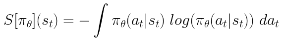
Entropy term

Finally, we encourage exploration with a small bonus on the entropy of the output distribution of the policy. We consider the standard entropy:

Entropy formula for the output distribution given by the policy model.

Implementation

Don’t worry if the theory still seems a bit shady. The implementation will hopefully make everything clear.

PPO-independent Code

Let’s start with the imports:

1from argparse import ArgumentParser
2
3import gym
4import numpy as np
5import wandb
6
7import torch
8import torch.nn as nn
9from torch.optim import Adam
10from torch.optim.lr_scheduler import LinearLR
11from torch.distributions.categorical import Categorical
12
13import pytorch_lightning as pl

The important hyper-parameters of PPO are the number of actors, horizon, epsilon, the number of epochs for each optimization phase, the learning rate, the discount factor gamma, and the constants that weigh the different loss terms c1 and c2. We collect these through the program arguments.

1def parse_args():
2"""Pareser program arguments"""
3# Parser
4parser = ArgumentParser()
5
6# Program arguments (default for Atari games)
7parser.add_argument("--max_iterations", type=int, help="Number of iterations of training", default=100)
8parser.add_argument("--n_actors", type=int, help="Number of actors for each update", default=8)
9parser.add_argument("--horizon", type=int, help="Number of timestamps for each actor", default=128)
10parser.add_argument("--epsilon", type=float, help="Epsilon parameter", default=0.1)
11parser.add_argument("--n_epochs", type=int, help="Number of training epochs per iteration", default=3)
12parser.add_argument("--batch_size", type=int, help="Batch size", default=32 * 8)
13parser.add_argument("--lr", type=float, help="Learning rate", default=2.5 * 1e-4)
14parser.add_argument("--gamma", type=float, help="Discount factor gamma", default=0.99)
15parser.add_argument("--c1", type=float, help="Weight for the value function in the loss function", default=1)
16parser.add_argument("--c2", type=float, help="Weight for the entropy bonus in the loss function", default=0.01)
17parser.add_argument("--n_test_episodes", type=int, help="Number of episodes to render", default=5)
18parser.add_argument("--seed", type=int, help="Randomizing seed for the experiment", default=0)
19
20# Dictionary with program arguments
21return vars(parser.parse_args())
22

Notice that, by default, the parameters are set as described in the paper. Ideally, our code should run on GPU if possible, so we create a simple utility function.

1def get_device():
2    """Gets the device (GPU if any) and logs the type"""
3    if torch.cuda.is_available():
4        device = torch.device("cuda")
5        print(f"Found GPU device: {torch.cuda.get_device_name(device)}")
6    else:
7        device = torch.device("cpu")
8        print("No GPU found: Running on CPU")
9    return device
10

When we apply RL, we typically have a buffer that stores states, actions, and rewards encountered by the current model. These are used to update our models. We create a utility function run_timestamps that will run a given model on a given environment for a fixed number of timestamps (re-setting the environment if the episode finishes). We also use an option render=False in case we just want to see how the trained model does.

1@torch.no_grad()
2def run_timestamps(env, model, timestamps=128, render=False, device="cpu"):
3    """Runs the given policy on the given environment for the given amount of timestamps.
4     Returns a buffer with state action transitions and rewards."""
5    buffer = []
6    state = env.reset()[0]
7
8    # Running timestamps and collecting state, actions, rewards and terminations
9    for ts in range(timestamps):
10        # Taking a step into the environment
11        model_input = torch.from_numpy(state).unsqueeze(0).to(device).float()
12        action, action_logits, value = model(model_input)
13        new_state, reward, terminated, truncated, info = env.step(action.item())
14
15        # Rendering / storing (s, a, r, t) in the buffer
16        if render:
17            env.render()
18        else:
19            buffer.append([model_input, action, action_logits, value, reward, terminated or truncated])
20
21        # Updating current state
22        state = new_state
23
24        # Resetting environment if episode terminated or truncated
25        if terminated or truncated:
26            state = env.reset()[0]
27
28    return buffer
29

The output of the function (when not rendering) is a buffer containing states, taken actions, action probabilities (logits), estimated critic’s values, rewards, and the termination state for the provided policy for each timestamp. Notice that the function uses the decorator @torch.no_grad(), so we will not need to store gradients for the actions taken during the interactions with the environment.

Code for PPO

Now that we got the trivial stuff out of the way, is time to implement the core algorithm.

Ideally, we would like our main function to look something like this:

1def main():
2    # Parsing program arguments
3    args = parse_args()
4    print(args)
5
6    # Setting seed
7    pl.seed_everything(args["seed"])
8
9    # Getting device
10    device = get_device()
11
12    # Creating environment (discrete action space)
13    env_name = "CartPole-v1"
14    env = gym.make(env_name)
15
16    # Creating the model, training it and rendering the result
17    # (We are missing this part 😅)
18    model = MyPPO(env.observation_space.shape, env.action_space.n).to(device)
19    training_loop(env, model, args)
20    model = load_best_model()
21    testing_loop(env, model)
22

We already got most of it. We just need to define the PPO model, the training, and the test functions.

The architecture of the PPO model is not the interesting part here. We just need two models (actor and critic) that will act in the environment. Of course, the model architecture plays a crucial role in harder tasks, but with the cart pole, we can be confident that some MLP will do the job.

Thus, we can create a MyPPO class that contains actor and critic models. Optionally, we may decide that part of the architecture between the two is shared. When running the forward method for some states, we return the sampled actions by the actor, the relative probabilities for each possible action (logits), and the critic’s estimated values for each state.

1class MyPPO(nn.Module):
2"""Implementation of a PPO model. The same backbone is used to get actor and critic values."""
3
4    def __init__(self, in_shape, n_actions, hidden_d=100, share_backbone=False):
5        # Super constructor
6        super(MyPPO, self).__init__()
7
8        # Attributes
9        self.in_shape = in_shape
10        self.n_actions = n_actions
11        self.hidden_d = hidden_d
12        self.share_backbone = share_backbone
13
14        # Shared backbone for policy and value functions
15        in_dim = np.prod(in_shape)
16
17        def to_features():
18            return nn.Sequential(
19                nn.Flatten(),
20                nn.Linear(in_dim, hidden_d),
21                nn.ReLU(),
22                nn.Linear(hidden_d, hidden_d),
23                nn.ReLU()
24            )
25
26        self.backbone = to_features() if self.share_backbone else nn.Identity()
27
28        # State action function
29        self.actor = nn.Sequential(
30            nn.Identity() if self.share_backbone else to_features(),
31            nn.Linear(hidden_d, hidden_d),
32            nn.ReLU(),
33            nn.Linear(hidden_d, n_actions),
34            nn.Softmax(dim=-1)
35        )
36
37        # Value function
38        self.critic = nn.Sequential(
39            nn.Identity() if self.share_backbone else to_features(),
40            nn.Linear(hidden_d, hidden_d),
41            nn.ReLU(),
42            nn.Linear(hidden_d, 1)
43        )
44
45    def forward(self, x):
46        features = self.backbone(x)
47        action = self.actor(features)
48        value = self.critic(features)
49        return Categorical(action).sample(), action, value
50

Notice that Categorical(action).sample() creates a categorical distribution with the action logits and samples from it one action (for each state).

Finally, we can take care of the actual algorithm in the training_loop function. As we know from the paper, the actual signature of the function should look something like this:

1def training_loop(env, model, max_iterations, n_actors, horizon, gamma, 
2    epsilon, n_epochs, batch_size, lr, c1, c2, device, env_name=""):
3    # TODO...
4

Here’s the pseudo-code provided in the paper for the PPO training procedure:

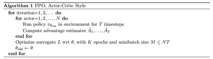
Pseudo code for PPO training provided in the original paper.

The pseudo-code for PPO is relatively simple: we simply collect interactions with the environment by multiple copies of our policy model (called actors) and use the objective previously defined to optimize both actor and critic networks.

Since we need to measure the cumulative rewards that we really obtained, we create a function that, given a buffer, replaces rewards at each timestamp with the cumulative rewards:

1def compute_cumulative_rewards(buffer, gamma):
2    """Given a buffer with states, policy action logits, rewards and terminations,
3    computes the cumulative rewards for each timestamp and substitutes them into the buffer."""
4    curr_rew = 0.
5
6    # Traversing the buffer on the reverse direction
7    for i in range(len(buffer) - 1, -1, -1):
8        r, t = buffer[i][-2], buffer[i][-1]
9
10        if t:
11            curr_rew = 0
12        else:
13            curr_rew = r + gamma * curr_rew
14
15        buffer[i][-2] = curr_rew
16
17    # Getting the average reward before normalizing (for logging and checkpointing)
18    avg_rew = np.mean([buffer[i][-2] for i in range(len(buffer))])
19
20    # Normalizing cumulative rewards
21    mean = np.mean([buffer[i][-2] for i in range(len(buffer))])
22    std = np.std([buffer[i][-2] for i in range(len(buffer))]) + 1e-6
23    for i in range(len(buffer)):
24        buffer[i][-2] = (buffer[i][-2] - mean) / std
25
26    return avg_rew
27

Notice that, in the end, we normalize the cumulative rewards. This is a standard trick to make the optimization problem easier and the training smoother.

Now that we can obtain a buffer with states, actions taken, actions probabilities, and cumulative rewards, we can write a function that, given a buffer, computes the three loss terms for our final objective:

1def get_losses(model, batch, epsilon, annealing, device="cpu"):
2    """Returns the three loss terms for a given model and a given batch and additional parameters"""
3    # Getting old data
4    n = len(batch)
5    states = torch.cat([batch[i][0] for i in range(n)])
6    actions = torch.cat([batch[i][1] for i in range(n)]).view(n, 1)
7    logits = torch.cat([batch[i][2] for i in range(n)])
8    values = torch.cat([batch[i][3] for i in range(n)])
9    cumulative_rewards = torch.tensor([batch[i][-2] for i in range(n)]).view(-1, 1).float().to(device)
10
11    # Computing predictions with the new model
12    _, new_logits, new_values = model(states)
13
14    # Loss on the state-action-function / actor (L_CLIP)
15    advantages = cumulative_rewards - values
16    margin = epsilon * annealing
17    ratios = new_logits.gather(1, actions) / logits.gather(1, actions)
18
19    l_clip = torch.mean(
20        torch.min(
21            torch.cat(
22                (ratios * advantages,
23                torch.clip(ratios, 1 - margin, 1 + margin) * advantages),
24                dim=1),
25            dim=1
26        ).values
27    )
28
29    # Loss on the value-function / critic (L_VF)
30    l_vf = torch.mean((cumulative_rewards - new_values) ** 2)
31
32    # Bonus for entropy of the actor
33    entropy_bonus = torch.mean(torch.sum(-new_logits * (torch.log(new_logits + 1e-5)), dim=1))
34
35    return l_clip, l_vf, entropy_bonus
36

Notice that, in practice, we use an annealing parameter that is set to 1 and linearly decayed towards 0 throughout the training. The idea is that as training progresses, we want our policy to change less and less. Also notice that the advantages variable is a simple difference between tensors for which we are not tracking gradients, unlike new_logits and new_values.

Now that we have a way to interact with the environment and store buffers, compute the (true) cumulative rewards and obtain the loss terms, we can write the final training loop:

1def training_loop(env, model, max_iterations, n_actors, horizon, gamma, epsilon, n_epochs, batch_size, lr,
2    c1, c2, device, env_name=""):
3    """Train the model on the given environment using multiple actors acting up to n timestamps."""
4
5    # Starting a new Weights & Biases run
6    wandb.init(project="Papers Re-implementations",
7    entity="peutlefaire",
8    name=f"PPO - {env_name}",
9    config={
10        "env": str(env),
11        "number of actors": n_actors,
12        "horizon": horizon,
13        "gamma": gamma,
14        "epsilon": epsilon,
15        "epochs": n_epochs,
16        "batch size": batch_size,
17        "learning rate": lr,
18        "c1": c1,
19        "c2": c2
20    })
21
22    # Training variables
23    max_reward = float("-inf")
24    optimizer = Adam(model.parameters(), lr=lr, maximize=True)
25    scheduler = LinearLR(optimizer, 1, 0, max_iterations * n_epochs)
26    anneals = np.linspace(1, 0, max_iterations)
27
28    # Training loop
29    for iteration in range(max_iterations):
30    buffer = []
31    annealing = anneals[iteration]
32
33    # Collecting timestamps for all actors with the current policy
34    for actor in range(1, n_actors + 1):
35    buffer.extend(run_timestamps(env, model, horizon, False, device))
36
37    # Computing cumulative rewards and shuffling the buffer
38    avg_rew = compute_cumulative_rewards(buffer, gamma)
39    np.random.shuffle(buffer)
40
41    # Running optimization for a few epochs
42    for epoch in range(n_epochs):
43    for batch_idx in range(len(buffer) // batch_size):
44    # Getting batch for this buffer
45    start = batch_size * batch_idx
46    end = start + batch_size if start + batch_size < len(buffer) else -1
47    batch = buffer[start:end]
48
49    # Zero-ing optimizers gradients
50    optimizer.zero_grad()
51
52    # Getting the losses
53    l_clip, l_vf, entropy_bonus = get_losses(model, batch, epsilon, annealing, device)
54
55    # Computing total loss and back-propagating it
56    loss = l_clip - c1 * l_vf + c2 * entropy_bonus
57    loss.backward()
58
59    # Optimizing
60    optimizer.step()
61    scheduler.step()
62
63    # Logging information to stdout
64    curr_loss = loss.item()
65    log = f"Iteration {iteration + 1} / {max_iterations}: "     f"Average Reward: {avg_rew:.2f}	"     f"Loss: {curr_loss:.3f} "     f"(L_CLIP: {l_clip.item():.1f} | L_VF: {l_vf.item():.1f} | L_bonus: {entropy_bonus.item():.1f})"
66    if avg_rew > max_reward:
67    torch.save(model.state_dict(), MODEL_PATH)
68    max_reward = avg_rew
69    log += " --> Stored model with highest average reward"
70    print(log)
71
72    # Logging information to W&B
73    wandb.log({
74    "loss (total)": curr_loss,
75    "loss (clip)": l_clip.item(),
76    "loss (vf)": l_vf.item(),
77    "loss (entropy bonus)": entropy_bonus.item(),
78    "average reward": avg_rew
79    })
80
81    # Finishing W&B session
82    wandb.finish()          
83

Finally, to see how the final model does, we use the following testing_loop function:

1def testing_loop(env, model, n_episodes, device):
2    """Runs the learned policy on the environment for n episodes"""
3    for _ in range(n_episodes):
4        run_timestamps(env, model, timestamps=128, render=True, device=device)
5

And our main program is simply:

1def main():
2    # Parsing program arguments
3    args = parse_args()
4    print(args)
5
6    # Setting seed
7    pl.seed_everything(args["seed"])
8
9    # Getting device
10    device = get_device()
11
12    # Creating environment (discrete action space)
13    env_name = "CartPole-v1"
14    env = gym.make(env_name)
15
16    # Creating the model (both actor and critic)
17    model = MyPPO(env.observation_space.shape, env.action_space.n).to(device)
18
19    # Training
20    training_loop(env, model, args["max_iterations"], args["n_actors"], args["horizon"], args["gamma"], args["epsilon"],
21                args["n_epochs"], args["batch_size"], args["lr"], args["c1"], args["c2"], device, env_name)
22
23    # Loading best model
24    model = MyPPO(env.observation_space.shape, env.action_space.n).to(device)
25    model.load_state_dict(torch.load(MODEL_PATH, map_location=device))
26
27    # Testing
28    env = gym.make(env_name, render_mode="human")
29    testing_loop(env, model, args["n_test_episodes"], device)
30    env.close()
31

And that’s all for the implementation! If you made it this far, congratulations. You pro now know how to implement the PPO algorithm.

Results

The Weights & Biases logs allow us to visualize the logged metrics and losses. In particular, we have access to plots of the loss and its terms and the average reward per iteration.

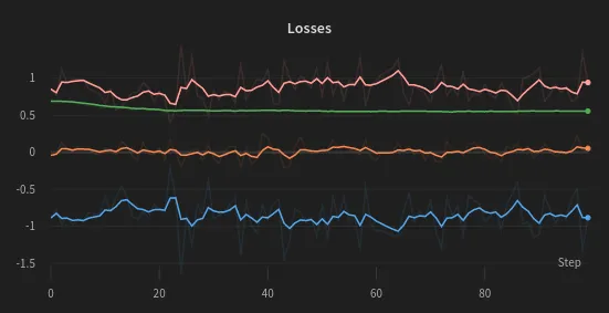
Training losses through training iterations. The total loss (blue) is the sum of L_CLIP (orange) minus the L_VF (pink) plus a small constant times the entropy bonus (green)

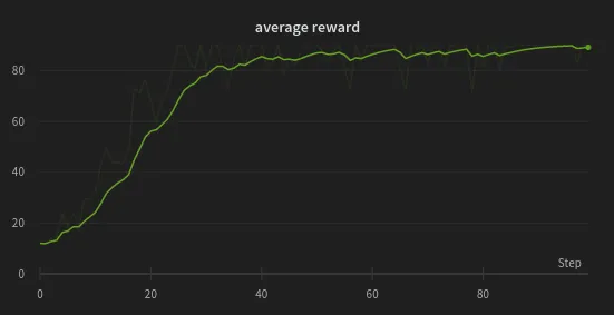
Average reward through iterations. PPO quickly learns to maximize the cumulative reward.

As the cart pole environment is not extremely challenging, our algorithm quickly finds a solution to the problem, maximizing the average reward after just ~20 steps. Also, since the environment only has 2 possible actions, the entropy term remains basically fixed.

Finally, here’s what we get if we render the final policy in action!

Trained PPO model balancing the cart pole

Conclusions

PPO is a state-of-the-art RL policy optimization (thus model-free) algorithm and as such, it can be virtually used in any environment. Also, PPO has a relatively simple objective function and relatively few hyper-parameters to be tuned.

If you would like to play with the algorithm on the fly, here’s a link to the Colab Notebook. You can find my personal up-to-date re-implementation of the PPO algorithm (as a .py file) under the GitHub repository. Feel free to play around with it or adapt it to your own project!

If you enjoyed this story, let me know! Feel free to reach out for further discussions. Wish you happy hacking with PPO ✌️