Published: 10.07.2022
Generating images with DDPMs: A PyTorch Implementation
Introduction
Denoising Diffusion Probabilistic Models (DDPM) are deep generative models that are recently getting a lot of attention due to their impressive performances. Brand new models like OpenAI’s DALL-E 2 and Google’s Imagen generators are based on DDPMs. They condition the generator on text such that it becomes then possible to generate photo-realistic images given an arbitrary string of text.
For example, inputting “A photo of a Shiba Inu dog with a backpack riding a bike. It is wearing sunglasses and a beach hat” to the new Imagen model and “a corgi’s head depicted as an explosion of a nebula” to the DALL-E 2 model produces the following images:
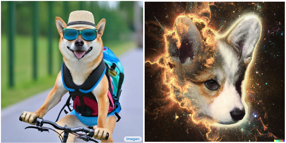
Image generated by Imagen (left) and DALL-E 2 (right)
These models are simply mind-blowing, but understanding how they work requires understanding the Original work of Ho et. al. “Denoise Diffusion Probabilistic Models”.
In this brief post, I will focus on creating from scratch (in PyTorch) a simple version of DDPM. In particular, I will be re-implementing the original paper by Ho. Et al. We will work with the classical and non-resource-hungry MNIST and Fashion-MNIST datasets, and try to generate images out of thin air. Let’s start with a little bit of theory.
Denoise Diffusion Probabilistic Models
Denoise Diffusion Probabilistic Models (DDPMs) first appeared in this paper.
The idea is quite simple: given a dataset of images, we add a little bit of noise step-by-step. With each step, the image becomes less and less clear, until all that is left is noise. This is called the “forward process”. Then, we learn a machine learning model that can undo each of such steps, and we call it the “backward process”. If we can successfully learn a backward process, we have a model that can generate images from pure random noise.
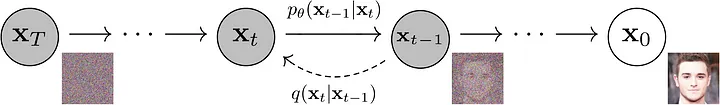
The main idea of DDPM: Map images x0 to more and more noisy images with probability distribution q. Then, learn the inverse function p parametrized by parameters theta. The image is taken from “Denoising DIffusion Probabilistic Models” by Ho et. al.
A step in the forward process consists in making the input image noisier (x at step t) by sampling from a multivariate gaussian distribution which mean is a scaled-down version of the previous image (x at step t-1) and which covariance matrix is diagonal and fixed. In other words, we perturb each pixel in the image independently by adding some normally distributed value.
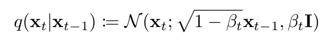
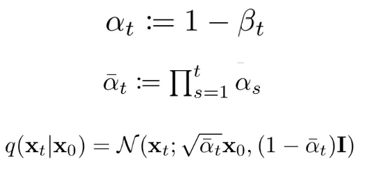
Forward process: we sample from a normal distribution which mean is a scaled version of the current image and which covariance matrix simply has all equal variance terms beta t.
For each step, there is a different coefficient beta that tells how much we are distorting the image in that step. The higher beta is, the more noise is added to the image. We are free to pick coefficients beta, but we should try to not have steps where too much noise is added all at once, and the overall forward process should be “smooth”. In the original work by Ho et. al., betas are put in a linear space from 0.0001 to 0.02.
A nice property of a gaussian distribution is that we can sample from it by adding to the mean vector a normally distributed noise vector scaled by the standard deviation. This results in:

Forward process but sampling is done by just adding the mean and scaling a normally distributed noise (epsilon) by the standard deviation.
We now know how to get the next sample in the forward process by just scaling what we already have and adding some scaled noise. If we now consider that the formula is recursive, we can write:
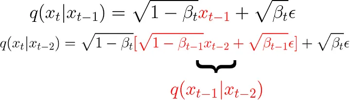
The formula of the forward process is recursive, so we can start expanding it.
If we keep doing this and do some simplifications, we can go all the way back and obtain a formula for getting the noisy sample at step t starting from the original non-noisy image x0:
The equation for the forward process that allows to directly get a desired noisy level starting from the original non-noisy image.
Great. Now no matter how many steps our forward process will have, we will always have a way to directly get the noisy image at step t directly from the original image.
For the backward process, we know our model should also work as a gaussian distribution, so we would just need the model to predict the distribution mean and standard deviation given the noisy image and time step. In practice, in this first paper on DDPMs the covariance matrix is kept fixed, so we only really want to predict the mean of the gaussian (given the noisy image and the time step we are at currently):

Backward process: we try to go back to a less noisy image (x at timestep t-1) using a gaussian distribution which mean is predicted by a model.
Now, it turns out that the optimal mean value to be predicted is just a function of terms that we are already familiar with:
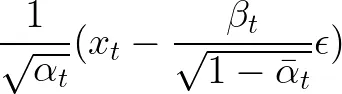
The optimal mean value to be predicted to reverse the noising process. Given the more noisy image at step t, we can make it less noisy by subtracting a scale of the added noise and applying a scaling afterwards.
So, we can further simplify our model and just predict the noise epsilon with a function of the noisy image and the time-step.
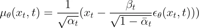
Our model just predicts the noise that was added, and we use this to recover a less noisy image using the information for the particular time step.
And our loss function is just going to be a scaled version of the Mean-Square Error (MSE) between the real noise that was added and the one predicted by our model
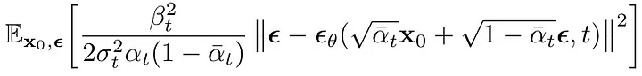
Final loss function. We minimize the MSE between the noises actually added to the images and the one predicted by the model. We do so for all images in our dataset and all time steps.
Once the model is trained (algorithm 1), we can use the denoising model to sample new images (algorithm 2).
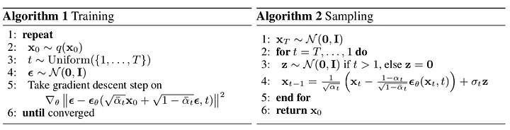
Training and sampling algorithms. Once the model is trained, we can use it to generate brand new samples starting from gaussian noise.
Let’s get coding
Now that we have a rough understanding of how diffusion models work, it’s time to implement something of our own. You can run the following code yourself in this Google Colab Notebook or with this GitHub repository.
As usual, imports are trivially our first step.
1# Import of libraries
2import random
3import imageio
4import numpy as np
5from argparse import ArgumentParser
6
7from tqdm.auto import tqdm
8import matplotlib.pyplot as plt
9
10import einops
11import torch
12import torch.nn as nn
13from torch.optim import Adam
14from torch.utils.data import DataLoader
15
16from torchvision.transforms import Compose, ToTensor, Lambda
17from torchvision.datasets.mnist import MNIST, FashionMNIST
18
19# Setting reproducibility
20SEED = 0
21random.seed(SEED)
22np.random.seed(SEED)
23torch.manual_seed(SEED)
24
25# Definitions
26STORE_PATH_MNIST = f"ddpm_model_mnist.pt"
27STORE_PATH_FASHION = f"ddpm_model_fashion.pt"
Next, we define a few parameters for our experiment. In particular, we decide if we want to run the training loop, whether we want to use the Fashion-MNIST dataset and some training hyper-parameters
1no_train = False
2fashion = True
3batch_size = 128
4n_epochs = 20
5lr = 0.001
6store_path = "ddpm_fashion.pt" if fashion else "ddpm_mnist.pt"
Next, we would really like to display images. Both the training images and those generated by the model are of interest to us. We write a utility function that given some images, will display a square (or as close as it gets) grid of sub-figures:
1def show_images(images, title=""):
2    """Shows the provided images as sub-pictures in a square"""
3
4    # Converting images to CPU numpy arrays
5    if type(images) is torch.Tensor:
6        images = images.detach().cpu().numpy()
7
8    # Defining number of rows and columns
9    fig = plt.figure(figsize=(8, 8))
10    rows = int(len(images) ** (1 / 2))
11    cols = round(len(images) / rows)
12
13    # Populating figure with sub-plots
14    idx = 0
15    for r in range(rows):
16        for c in range(cols):
17            fig.add_subplot(rows, cols, idx + 1)
18
19            if idx < len(images):
20                plt.imshow(images[idx][0], cmap="gray")
21                idx += 1
22    fig.suptitle(title, fontsize=30)
23
24    # Showing the figure
25    plt.show()
To test this utility function, we load our dataset and show the first batch. Important: Images must be normalized in the range [-1, 1], as our network will have to predict noise values that are normally distributed:
1# Shows the first batch of images
2def show_first_batch(loader):
3    for batch in loader:
4        show_images(batch[0], "Images in the first batch")
5 break1# Loading the data (converting each image into a tensor and normalizing between [-1, 1])
2transform = Compose([
3 ToTensor(),
4 Lambda(lambda x: (x - 0.5) * 2)]
5)
6ds_fn = FashionMNIST if fashion else MNIST
7dataset = ds_fn("./datasets", download=True, train=True, transform=transform)
8loader = DataLoader(dataset, batch_size, shuffle=True)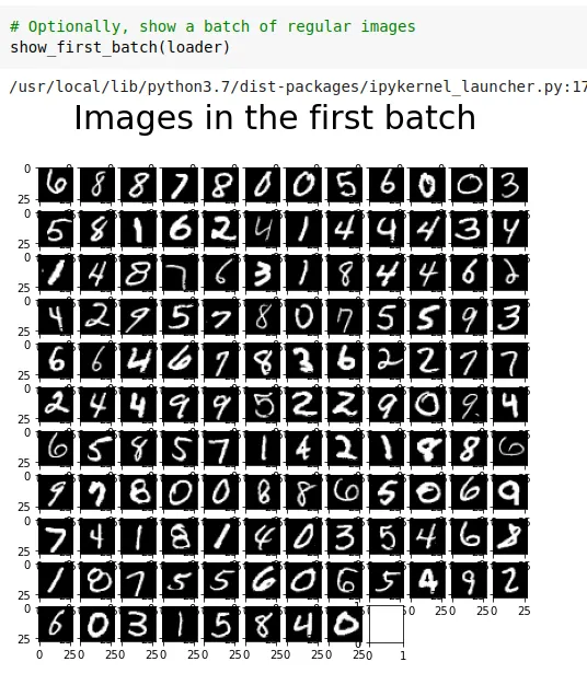
Images in our first batch. If you kept the same randomizing seed, you should get the exact same batch.
Great! Now that we have this nice utility function, we will use it for images generated by our model later on as well. Before we start actually dealing with the DDPM model, we will just get a GPU device from colab (typically a Tesla T4 for non colab-pro users):
1# Getting device
2device = torch.device('cuda' if torch.cuda.is_available() else 'cpu')
3print(f"Using device: {device}	" + (f"{torch.cuda.get_device_name(device)}" if torch.cuda.is_available() else "CPU"))
The DDPM Model
Now that we got the trivial stuff out of the way, it’s time to work on the DDPM. We will create a MyDDPM PyTorch module that will be responsible for storing betas and alphas values and applying the forward process. For the backward process instead, the MyDDPM module will simply rely on a network used for constructing the DDPM:
1# DDPM class
2class MyDDPM(nn.Module):
3    def __init__(self, network, n_steps=200, min_beta=10 ** -4, max_beta=0.02, device=None, image_chw=(1, 28, 28)):
4        super(MyDDPM, self).__init__()
5        self.n_steps = n_steps
6        self.device = device
7        self.image_chw = image_chw
8        self.network = network.to(device)
9        self.betas = torch.linspace(min_beta, max_beta, n_steps).to(
10            device)  # Number of steps is typically in the order of thousands
11        self.alphas = 1 - self.betas
12        self.alpha_bars = torch.tensor([torch.prod(self.alphas[:i + 1]) for i in range(len(self.alphas))]).to(device)
13
14    def forward(self, x0, t, eta=None):
15        # Make input image more noisy (we can directly skip to the desired step)
16        n, c, h, w = x0.shape
17        a_bar = self.alpha_bars[t]
18
19        if eta is None:
20            eta = torch.randn(n, c, h, w).to(self.device)
21
22        noisy = a_bar.sqrt().reshape(n, 1, 1, 1) * x0 + (1 - a_bar).sqrt().reshape(n, 1, 1, 1) * eta
23        return noisy
24
25    def backward(self, x, t):
26        # Run each image through the network for each timestep t in the vector t.
27        # The network returns its estimation of the noise that was added.
28        return self.network(x, t)
Note that the forward process is independent of the network used to denoise, so technically we could already visualize its effect. At the same time, we can also create a utility function that applies Algorithm 2 (sampling procedure) to generate new images. We do so with two DDPM’s specific utility functions:
1def show_forward(ddpm, loader, device):
2    # Showing the forward process
3    for batch in loader:
4        imgs = batch[0]
5
6        show_images(imgs, "Original images")
7
8        for percent in [0.25, 0.5, 0.75, 1]:
9            show_images(
10                ddpm(imgs.to(device),
11                     [int(percent * ddpm.n_steps) - 1 for _ in range(len(imgs))]),
12                f"DDPM Noisy images {int(percent * 100)}%"
13            )
14        break
To generate images, we start with random noise and let t go from T back to 0. At each step, we estimate the noise as eta_theta and apply the denoising function. Finally, extra noise is added as in Langevin dynamics.
1def generate_new_images(ddpm, n_samples=16, device=None, frames_per_gif=100, gif_name="sampling.gif", c=1, h=28, w=28):
2    """Given a DDPM model, a number of samples to be generated and a device, returns some newly generated samples"""
3    frame_idxs = np.linspace(0, ddpm.n_steps, frames_per_gif).astype(np.uint)
4    frames = []
5
6    with torch.no_grad():
7        if device is None:
8            device = ddpm.device
9
10        # Starting from random noise
11        x = torch.randn(n_samples, c, h, w).to(device)
12
13        for idx, t in enumerate(list(range(ddpm.n_steps))[::-1]):
14            # Estimating noise to be removed
15            time_tensor = (torch.ones(n_samples, 1) * t).to(device).long()
16            eta_theta = ddpm.backward(x, time_tensor)
17
18            alpha_t = ddpm.alphas[t]
19            alpha_t_bar = ddpm.alpha_bars[t]
20
21            # Partially denoising the image
22            x = (1 / alpha_t.sqrt()) * (x - (1 - alpha_t) / (1 - alpha_t_bar).sqrt() * eta_theta)
23
24            if t > 0:
25                z = torch.randn(n_samples, c, h, w).to(device)
26
27                # Option 1: sigma_t squared = beta_t
28                beta_t = ddpm.betas[t]
29                sigma_t = beta_t.sqrt()
30
31                # Option 2: sigma_t squared = beta_tilda_t
32                # prev_alpha_t_bar = ddpm.alpha_bars[t-1] if t > 0 else ddpm.alphas[0]
33                # beta_tilda_t = ((1 - prev_alpha_t_bar)/(1 - alpha_t_bar)) * beta_t
34                # sigma_t = beta_tilda_t.sqrt()
35
36                # Adding some more noise like in Langevin Dynamics fashion
37                x = x + sigma_t * z
38
39            # Adding frames to the GIF
40            if idx in frame_idxs or t == 0:
41                # Putting digits in range [0, 255]
42                normalized = x.clone()
43                for i in range(len(normalized)):
44                    normalized[i] -= torch.min(normalized[i])
45                    normalized[i] *= 255 / torch.max(normalized[i])
46
47                # Reshaping batch (n, c, h, w) to be a (as much as it gets) square frame
48                frame = einops.rearrange(normalized, "(b1 b2) c h w -> (b1 h) (b2 w) c", b1=int(n_samples ** 0.5))
49                frame = frame.cpu().numpy().astype(np.uint8)
50
51                # Rendering frame
52                frames.append(frame)
53
54    # Storing the gif
55    with imageio.get_writer(gif_name, mode="I") as writer:
56        for idx, frame in enumerate(frames):
57            writer.append_data(frame)
58            if idx == len(frames) - 1:
59                for _ in range(frames_per_gif // 3):
60                    writer.append_data(frames[-1])
61    return x
Everything that concerns DDPM is on the table now. We simply need to define the model that will actually do the job of predicting the noise in the image given the image and the current time step. To do that, we will create a custom U-Net model. It goes without saying that you are free to use any other model of your choice.
The U-Net
We start the creation of our U-Net by creating a block that will keep spatial dimensionality unchanged. This block will be used at every level of our U-Net.
1class MyBlock(nn.Module):
2    def __init__(self, shape, in_c, out_c, kernel_size=3, stride=1, padding=1, activation=None, normalize=True):
3        super(MyBlock, self).__init__()
4        self.ln = nn.LayerNorm(shape)
5        self.conv1 = nn.Conv2d(in_c, out_c, kernel_size, stride, padding)
6        self.conv2 = nn.Conv2d(out_c, out_c, kernel_size, stride, padding)
7        self.activation = nn.SiLU() if activation is None else activation
8        self.normalize = normalize
9
10    def forward(self, x):
11        out = self.ln(x) if self.normalize else x
12        out = self.conv1(out)
13        out = self.activation(out)
14        out = self.conv2(out)
15        out = self.activation(out)
16        return out
The tricky thing in DDPMs is that our image-to-image model has to be conditioned on the current time step. To do so in practice, we use sinusoidal embedding and one-layer MLPs. The resulting tensors will be added channel-wise to the input of the network through every level of the U-Net.
1def sinusoidal_embedding(n, d):
2    # Returns the standard positional embedding
3    embedding = torch.zeros(n, d)
4    wk = torch.tensor([1 / 10_000 ** (2 * j / d) for j in range(d)])
5    wk = wk.reshape((1, d))
6    t = torch.arange(n).reshape((n, 1))
7    embedding[:,::2] = torch.sin(t * wk[:,::2])
8    embedding[:,1::2] = torch.cos(t * wk[:,::2])
9
10    return embedding
We create a small utility function that creates a one-layer MLP which will be used to map positional embeddings.
1def _make_te(self, dim_in, dim_out):
2    return nn.Sequential(
3      nn.Linear(dim_in, dim_out),
4      nn.SiLU(),
5      nn.Linear(dim_out, dim_out)
6    )
Now that we know how to deal with the time information, we can create a custom U-Net network. We will have 3 down-sample parts, a bottleneck in the middle of the network, and 3 up-sample steps with the usual U-Net residual connections (concatenations).
1class MyUNet(nn.Module):
2    def __init__(self, n_steps=1000, time_emb_dim=100):
3        super(MyUNet, self).__init__()
4
5        # Sinusoidal embedding
6        self.time_embed = nn.Embedding(n_steps, time_emb_dim)
7        self.time_embed.weight.data = sinusoidal_embedding(n_steps, time_emb_dim)
8        self.time_embed.requires_grad_(False)
9
10        # First half
11        self.te1 = self._make_te(time_emb_dim, 1)
12        self.b1 = nn.Sequential(
13            MyBlock((1, 28, 28), 1, 10),
14            MyBlock((10, 28, 28), 10, 10),
15            MyBlock((10, 28, 28), 10, 10)
16        )
17        self.down1 = nn.Conv2d(10, 10, 4, 2, 1)
18
19        self.te2 = self._make_te(time_emb_dim, 10)
20        self.b2 = nn.Sequential(
21            MyBlock((10, 14, 14), 10, 20),
22            MyBlock((20, 14, 14), 20, 20),
23            MyBlock((20, 14, 14), 20, 20)
24        )
25        self.down2 = nn.Conv2d(20, 20, 4, 2, 1)
26
27        self.te3 = self._make_te(time_emb_dim, 20)
28        self.b3 = nn.Sequential(
29            MyBlock((20, 7, 7), 20, 40),
30            MyBlock((40, 7, 7), 40, 40),
31            MyBlock((40, 7, 7), 40, 40)
32        )
33        self.down3 = nn.Sequential(
34            nn.Conv2d(40, 40, 2, 1),
35            nn.SiLU(),
36            nn.Conv2d(40, 40, 4, 2, 1)
37        )
38
39        # Bottleneck
40        self.te_mid = self._make_te(time_emb_dim, 40)
41        self.b_mid = nn.Sequential(
42            MyBlock((40, 3, 3), 40, 20),
43            MyBlock((20, 3, 3), 20, 20),
44            MyBlock((20, 3, 3), 20, 40)
45        )
46
47        # Second half
48        self.up1 = nn.Sequential(
49            nn.ConvTranspose2d(40, 40, 4, 2, 1),
50            nn.SiLU(),
51            nn.ConvTranspose2d(40, 40, 2, 1)
52        )
53
54        self.te4 = self._make_te(time_emb_dim, 80)
55        self.b4 = nn.Sequential(
56            MyBlock((80, 7, 7), 80, 40),
57            MyBlock((40, 7, 7), 40, 20),
58            MyBlock((20, 7, 7), 20, 20)
59        )
60
61        self.up2 = nn.ConvTranspose2d(20, 20, 4, 2, 1)
62        self.te5 = self._make_te(time_emb_dim, 40)
63        self.b5 = nn.Sequential(
64            MyBlock((40, 14, 14), 40, 20),
65            MyBlock((20, 14, 14), 20, 10),
66            MyBlock((10, 14, 14), 10, 10)
67        )
68
69        self.up3 = nn.ConvTranspose2d(10, 10, 4, 2, 1)
70        self.te_out = self._make_te(time_emb_dim, 20)
71        self.b_out = nn.Sequential(
72            MyBlock((20, 28, 28), 20, 10),
73            MyBlock((10, 28, 28), 10, 10),
74            MyBlock((10, 28, 28), 10, 10, normalize=False)
75        )
76
77        self.conv_out = nn.Conv2d(10, 1, 3, 1, 1)
78
79    def forward(self, x, t):
80        # x is (N, 2, 28, 28) (image with positional embedding stacked on channel dimension)
81        t = self.time_embed(t)
82        n = len(x)
83        out1 = self.b1(x + self.te1(t).reshape(n, -1, 1, 1))  # (N, 10, 28, 28)
84        out2 = self.b2(self.down1(out1) + self.te2(t).reshape(n, -1, 1, 1))  # (N, 20, 14, 14)
85        out3 = self.b3(self.down2(out2) + self.te3(t).reshape(n, -1, 1, 1))  # (N, 40, 7, 7)
86
87        out_mid = self.b_mid(self.down3(out3) + self.te_mid(t).reshape(n, -1, 1, 1))  # (N, 40, 3, 3)
88
89        out4 = torch.cat((out3, self.up1(out_mid)), dim=1)  # (N, 80, 7, 7)
90        out4 = self.b4(out4 + self.te4(t).reshape(n, -1, 1, 1))  # (N, 20, 7, 7)
91
92        out5 = torch.cat((out2, self.up2(out4)), dim=1)  # (N, 40, 14, 14)
93        out5 = self.b5(out5 + self.te5(t).reshape(n, -1, 1, 1))  # (N, 10, 14, 14)
94
95        out = torch.cat((out1, self.up3(out5)), dim=1)  # (N, 20, 28, 28)
96        out = self.b_out(out + self.te_out(t).reshape(n, -1, 1, 1))  # (N, 1, 28, 28)
97
98        out = self.conv_out(out)
99
100        return out
101
102    def _make_te(self, dim_in, dim_out):
103        return nn.Sequential(
104            nn.Linear(dim_in, dim_out),
105            nn.SiLU(),
106            nn.Linear(dim_out, dim_out)
107        )
Now that we defined our denoising network, we can proceed to instantiate a DDPM model and play with some visualizations.
Some visualizations
We instantiate the DDPM model using our custom U-Net as follows.
1# Defining model
2n_steps, min_beta, max_beta = 1000, 10 ** -4, 0.02  # Originally used by the authors
3ddpm = MyDDPM(MyUNet(n_steps), n_steps=n_steps, min_beta=min_beta, max_beta=max_beta, device=device)
4
Let’s check what the forward process looks like:
1# Optionally, show the diffusion (forward) process
2show_forward(ddpm, loader, device)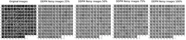
Result of running the forward process. Images get noisier and noisier with each step until just noise is left.
We have not trained the model yet, but we can already use the function that allows us to generate new images and see what happens:
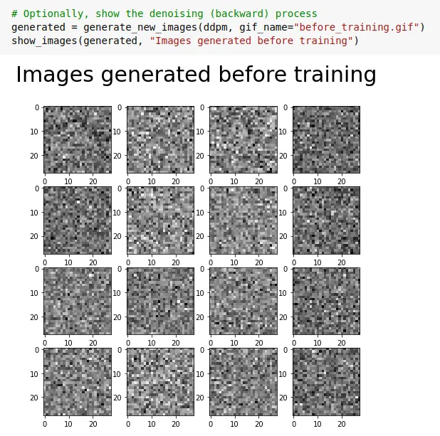
Generating new images with a non-trained model. Noise is produced.
Not surprisingly, nothing happens when we do so. However, we will re-use this same method later on when the model will be finished training.
Training loop
We now implement Algorithm 1 to learn a model that will know how to denoise images. This corresponds to our training loop.
1def training_loop(ddpm, loader, n_epochs, optim, device, display=False, store_path="ddpm_model.pt"):
2    mse = nn.MSELoss()
3    best_loss = float("inf")
4    n_steps = ddpm.n_steps
5
6    for epoch in tqdm(range(n_epochs), desc=f"Training progress", colour="#00ff00"):
7        epoch_loss = 0.0
8        for step, batch in enumerate(tqdm(loader, leave=False, desc=f"Epoch {epoch + 1}/{n_epochs}", colour="#005500")):
9            # Loading data
10            x0 = batch[0].to(device)
11            n = len(x0)
12
13            # Picking some noise for each of the images in the batch, a timestep and the respective alpha_bars
14            eta = torch.randn_like(x0).to(device)
15            t = torch.randint(0, n_steps, (n,)).to(device)
16
17            # Computing the noisy image based on x0 and the time-step (forward process)
18            noisy_imgs = ddpm(x0, t, eta)
19
20            # Getting model estimation of noise based on the images and the time-step
21            eta_theta = ddpm.backward(noisy_imgs, t.reshape(n, -1))
22
23            # Optimizing the MSE between the noise plugged and the predicted noise
24            loss = mse(eta_theta, eta)
25            optim.zero_grad()
26            loss.backward()
27            optim.step()
28
29            epoch_loss += loss.item() * len(x0) / len(loader.dataset)
30
31        # Display images generated at this epoch
32        if display:
33            show_images(generate_new_images(ddpm, device=device), f"Images generated at epoch {epoch + 1}")
34
35        log_string = f"Loss at epoch {epoch + 1}: {epoch_loss:.3f}"
36
37        # Storing the model
38        if best_loss > epoch_loss:
39            best_loss = epoch_loss
40            torch.save(ddpm.state_dict(), store_path)
41            log_string += " --> Best model ever (stored)"
42
43        print(log_string)
As you can see, in our training loop we simply sample some images and some random time steps for each of them. We then make them noisy with the forward process and run the backward process on those noisy images. The MSE between the actual noise added and the one predicted by the model is optimized.

Training takes roughly 24 seconds per epoch. With 20 epochs, it takes roughly 8 minutes to train a DDPM model.
By default, I set the training epochs to 20 as it takes 24 seconds per epoch (total of roughly 8 minutes to train). Note that it is possible to obtain even better performances with more epochs, a better U-Net, and other tricks. In this post, I omit those for simplicity.
Testing the model
Now that the job is done, we can simply enjoy the results. We load the best model obtained during training according to the MSE loss function, set it to evaluation mode and use it to generate new samples
1# Loading the trained model
2best_model = MyDDPM(MyUNet(), n_steps=n_steps, device=device)
3best_model.load_state_dict(torch.load(store_path, map_location=device))
4best_model.eval()
5print("Model loaded")1print("Generating new images")
2generated = generate_new_images(
3 best_model,
4 n_samples=100,
5 device=device,
6 gif_name="fashion.gif" if fashion else "mnist.gif"
7 )
8show_images(generated, "Final result")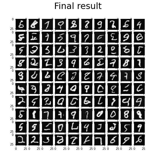
Final result on the MNIST dataset.
The cherry on the cake is the fact that our generation function automatically creates a nice gif of the diffusion process. We visualize that gif in Colab with the following command:
1from IPython.display import Image
2Image(open("fashion.gif" if fashion else "mnist.gif", "rb").read())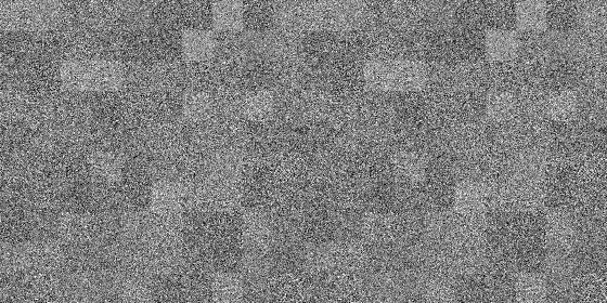
And we are done! We finally have our DDPM model working!
Further Improvements
Further improvements have been made, as to allow the generation of higher resolution images, accelerate sampling or obtain better sample quality and likelihood. Imagen and DALL-E 2 models are based on improved versions of the original DDPMs.
More References
For more references regarding DDPMs, I strongly recommend reading the outstanding post by Lilian Weng and Niels Rogge and Kashif Rasul’s amazing Hugging Face Blog. Other authors are also mentioned at the end of the Colab Notebook.
Conclusion
Diffusion models are generative models that learn to denoise images iteratively. Starting from some noise is then possible to ask the model to de-noise the sample until some realistic image is obtained.
We created a DDPM from scratch in PyTorch and had it learn to de-noise MNIST / Fashion-MNIST images. The model, after training, was finally capable of generating new images out of random noise. Quite magical, right?
The Colab Notebook with the shown implementation is freely accessible at this link, while the GitHub repository contains .py files. If you feel like something is unclear, don’t hesitate to contact me directly! I’d be glad to discuss it with you.