Published: 03.02.2022
Vision Transformers from Scratch (PyTorch): A step-by-step guide
Introduction
Vision Transformers (ViT), since their introduction by Dosovitskiy et. al. in 2020, have dominated the field of Computer Vision, obtaining state-of-the-art performance in image classification first, and later on in other tasks as well.
However, unlike other architectures, they are a bit harder to grasp, particularly if you are not already familiar with the Transformer model used in Natural Language Processing (NLP).
If you are into Computer Vision (CV) and are still unfamiliar with the ViT model, don't worry! So was I!
In this brief piece of text, I will show you how I implemented my first ViT from scratch (using PyTorch), and I will guide you through some debugging that will help you better visualize what exactly happens in a ViT.
While this article is specific to ViT, the concepts you will find here, such as the Multi-headed Self Attention (MSA) block, are present and currently very relevant in various sub-fields of AI, such as CV, NLP, etc…
Defining the task
Since the goal is just learning more about the ViT architecture, it is wise to pick an easy and well-known task and dataset. In our case, the task is the image classification for the popular MNIST dataset by the great LeCun et. al.
If you didn’t already know, MNIST is a dataset of hand-written digits ([0–9]) all contained in 28x28 binary pixels images. The task is referred to as trivial for today's algorithms, so we can expect that a correct implementation will perform well.
Let’s start with the imports then:
1import numpy as np
2
3from tqdm import tqdm, trange
4
5import torch
6import torch.nn as nn
7from torch.optim import Adam
8from torch.nn import CrossEntropyLoss
9from torch.utils.data import DataLoader
10
11from torchvision.transforms import ToTensor
12from torchvision.datasets.mnist import MNIST
13
14np.random.seed(0)
15torch.manual_seed(0)
16
Let’s create a main function that prepares the MNIST dataset, instantiates a model, and trains it for 5 epochs. After that, the loss and accuracy are measured on the test set.
1def main():
2    # Loading data
3    transform = ToTensor()
4
5    train_set = MNIST(root='./../datasets', train=True, download=True, transform=transform)
6    test_set = MNIST(root='./../datasets', train=False, download=True, transform=transform)
7
8    train_loader = DataLoader(train_set, shuffle=True, batch_size=128)
9    test_loader = DataLoader(test_set, shuffle=False, batch_size=128)
10
11    # Defining model and training options
12    device = torch.device("cuda" if torch.cuda.is_available() else "cpu")
13    print("Using device: ", device, f"({torch.cuda.get_device_name(device)})" if torch.cuda.is_available() else "")
14    model = MyViT((1, 28, 28), n_patches=7, n_blocks=2, hidden_d=8, n_heads=2, out_d=10).to(device)
15    N_EPOCHS = 5
16    LR = 0.005
17
18    # Training loop
19    optimizer = Adam(model.parameters(), lr=LR)
20    criterion = CrossEntropyLoss()
21    for epoch in trange(N_EPOCHS, desc="Training"):
22        train_loss = 0.0
23        for batch in tqdm(train_loader, desc=f"Epoch {epoch + 1} in training", leave=False):
24            x, y = batch
25            x, y = x.to(device), y.to(device)
26            y_hat = model(x)
27            loss = criterion(y_hat, y)
28
29            train_loss += loss.detach().cpu().item() / len(train_loader)
30
31            optimizer.zero_grad()
32            loss.backward()
33            optimizer.step()
34
35        print(f"Epoch {epoch + 1}/{N_EPOCHS} loss: {train_loss:.2f}")
36
37    # Test loop
38    with torch.no_grad():
39        correct, total = 0, 0
40        test_loss = 0.0
41        for batch in tqdm(test_loader, desc="Testing"):
42            x, y = batch
43            x, y = x.to(device), y.to(device)
44            y_hat = model(x)
45            loss = criterion(y_hat, y)
46            test_loss += loss.detach().cpu().item() / len(test_loader)
47
48            correct += torch.sum(torch.argmax(y_hat, dim=1) == y).detach().cpu().item()
49            total += len(x)
50        print(f"Test loss: {test_loss:.2f}")
51        print(f"Test accuracy: {correct / total * 100:.2f}%")
52
Now that we have this template, from now on, we can just focus on the model (ViT) that will have to classify the images with shape (N x 1 x 28 x 28).
Let’s start by defining an empty nn.Module. We will then fill this class step by step.
1class MyViT(nn.Module):
2    def __init__(self):
3        # Super constructor
4        super(MyViT, self).__init__()
5
6    def forward(self, images):
7        pass
8
Forward pass
As Pytorch, as well as most DL frameworks, provides autograd computations, we are only concerned with implementing the forward pass of the ViT model. Since we have defined the optimizer of the model already, the framework will take care of back-propagating gradients and training the model’s parameters.
While implementing a new model, I like to keep a picture of the architecture on some tab. Here’s our reference picture for the ViT from Bazi et. al (2021):
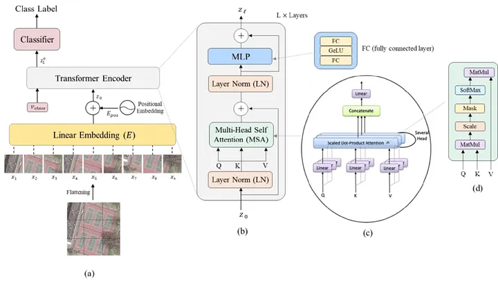
The architecture of the ViT with specific details on the transformer encoder and the MSA block. Keep this picture in mind. Picture from Bazi et. al.
By the picture, we see that the input image (a) is “cut” into sub-images equally sized.
Each such sub-image goes through a linear embedding. From then on, each sub-image is just a one-dimensional vector.
A positional embedding is then added to these vectors (tokens). The positional embedding allows the network to know where each sub-image is positioned originally in the image. Without this information, the network would not be able to know where each such image would be placed, leading to potentially wrong predictions!
These tokens are then passed, together with a special classification token, to the transformer encoders blocks, were each is composed of : A Layer Normalization (LN), followed by a Multi-head Self Attention (MSA) and a residual connection. Then a second LN, a Multi-Layer Perceptron (MLP), and again a residual connection. These blocks are connected back-to-back.
Finally, a classification MLP block is used for the final classification only on the special classification token, which by the end of this process has global information about the picture.
Let’s build the ViT in 6 main steps.
Step 1: Patchifying and the linear mapping
The transformer encoder was developed with sequence data in mind, such as English sentences. However, an image is not a sequence. It is just, uhm… an image… So how do we “sequencify” an image? We break it into multiple sub-images and map each sub-image to a vector!
We do so by simply reshaping our input, which has size (N, C, H, W) (in our example (N, 1, 28, 28)), to size (N, #Patches, Patch dimensionality), where the dimensionality of a patch is adjusted accordingly.
In this example, we break each (1, 28, 28) into 7x7 patches (hence, each of size 4x4). That is, we are going to obtain 7x7=49 sub-images out of a single image.
Thus, we reshape input (N, 1, 28, 28) to (N, PxP, HxC/P x WxC/P) = (N, 49, 16)
Notice that, while each patch is a picture of size 1x4x4, we flatten it to a 16-dimensional vector. Also, in this case, we only had a single color channel. If we had multiple color channels, those would also have been flattened into the vector.
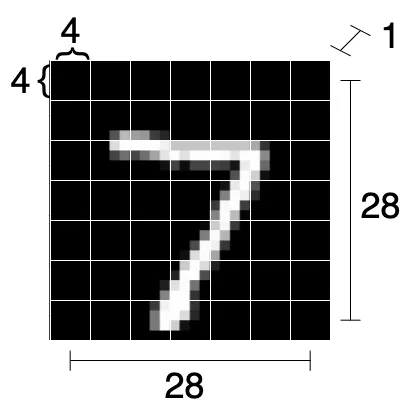
Raffiguration of how an image is split into patches. The 1x28x28 image is split into 49 (7x7) patches, each of size 16 (4x4x1)
We modify our MyViT class to implement the patchifying only. We create a method that does the operation from scratch. Notice that this is an inefficient way to carry out the operation, but the code is intuitive for learning about the core concept.
1def patchify(images, n_patches):
2    n, c, h, w = images.shape
3
4    assert h == w, "Patchify method is implemented for square images only"
5
6    patches = torch.zeros(n, n_patches ** 2, h * w * c // n_patches ** 2)
7    patch_size = h // n_patches
8
9    for idx, image in enumerate(images):
10        for i in range(n_patches):
11            for j in range(n_patches):
12                patch = image[:, i * patch_size: (i + 1) * patch_size, j * patch_size: (j + 1) * patch_size]
13                patches[idx, i * n_patches + j] = patch.flatten()
14    return patches
151class MyViT(nn.Module):
2 def __init__(self, chw=(1, 28, 28), n_patches=7):
3 # Super constructor
4 super(MyViT, self).__init__()
5
6 # Attributes
7 self.chw = chw # (C, H, W)
8 self.n_patches = n_patches
9
10 assert chw[1] % n_patches == 0, "Input shape not entirely divisible by number of patches"
11 assert chw[2] % n_patches == 0, "Input shape not entirely divisible by number of patches"
12
13 def forward(self, images):
14 patches = patchify(images, self.n_patches)
15 return patches
16The class constructor now lets the class know the size of our input images (number of channels, height and width). Note that in this implementation, the n_patches variable is the number of patches that we will find both in width and height (in our case it’s 7 because we break the image into 7x7 patches).
We can test the functioning of our class with a simple main program:
1if __name__ == '__main__':
2    # Current model
3    model = MyViT(
4        chw=(1, 28, 28),
5        n_patches=7
6    )
7
8    x = torch.randn(7, 1, 28, 28) # Dummy images
9    print(model(x).shape) # torch.Size([7, 49, 16])
10
Now that we have our flattened patches, we can map each of them through a Linear mapping. While each patch was a 4x4=16 dimensional vector, the linear mapping can map to any arbitrary vector size. Thus, we add a parameter to our class constructor, called hidden_d for ‘hidden dimension’.
In this example, we will use a hidden dimension of 8, but in principle, any number can be put here. We will thus be mapping each 16-dimensional patch to an 8-dimensional patch.
We simply create a nn.Linear layer and call it in our forward function.
1class MyViT(nn.Module):
2    def __init__(self, chw=(1, 28, 28), n_patches=7):
3        # Super constructor
4        super(MyViT, self).__init__()
5
6        # Attributes
7        self.chw = chw # (C, H, W)
8        self.n_patches = n_patches
9
10        assert chw[1] % n_patches == 0, "Input shape not entirely divisible by number of patches"
11        assert chw[2] % n_patches == 0, "Input shape not entirely divisible by number of patches"
12        self.patch_size = (chw[1] / n_patches, chw[2] / n_patches)
13
14        # 1) Linear mapper
15        self.input_d = int(chw[0] * self.patch_size[0] * self.patch_size[1])
16        self.linear_mapper = nn.Linear(self.input_d, self.hidden_d)
17
18    def forward(self, images):
19        patches = patchify(images, self.n_patches)
20        tokens = self.linear_mapper(patches)
21        return tokens
22
Notice that we run an (N, 49, 16) tensor through a (16, 8) linear mapper (or matrix). The linear operation only happens on the last dimension.
Step 2: Adding the classification token
If you look closely at the architecture picture, you will notice that also a v_class token is passed to the Transformer Encoder. What’s this?
Simply put, this is a special token that we add to our model that has the role of capturing information about the other tokens. This will happen with the MSA block (later on). When information about all other tokens will be present here, we will be able to classify the image using only this special token. The initial value of the special token (the one fed to the transformer encoder) is a parameter of the model that needs to be learned.
This is a cool concept of transformers! If we wanted to do another downstream task, we would just need to add another special token for the other downstream task (for example, classifying a digit as higher than 5 or lower) and a classifier that takes as input this new token. Clever, right?
We can now add a parameter to our model and convert our (N, 49, 8) tokens tensor to an (N, 50, 8) tensor (we add the special token to each sequence).
1class MyViT(nn.Module):
2    def __init__(self, chw=(1, 28, 28), n_patches=7):
3        # Super constructor
4        super(MyViT, self).__init__()
5
6        # Attributes
7        self.chw = chw # (C, H, W)
8        self.n_patches = n_patches
9
10        assert chw[1] % n_patches == 0, "Input shape not entirely divisible by number of patches"
11        assert chw[2] % n_patches == 0, "Input shape not entirely divisible by number of patches"
12        self.patch_size = (chw[1] / n_patches, chw[2] / n_patches)
13
14        # 1) Linear mapper
15        self.input_d = int(chw[0] * self.patch_size[0] * self.patch_size[1])
16        self.linear_mapper = nn.Linear(self.input_d, self.hidden_d)
17
18        # 2) Learnable classifiation token
19        self.class_token = nn.Parameter(torch.rand(1, self.hidden_d))
20
21    def forward(self, images):
22        patches = patchify(images, self.n_patches)
23        tokens = self.linear_mapper(patches)
24
25        # Adding classification token to the tokens
26        tokens = torch.stack([torch.vstack((self.class_token, tokens[i])) for i in range(len(tokens))])
27        return tokens
28
Notice that the classification token is put as the first token of each sequence. This will be important to keep in mind when we will then retrieve the classification token to feed to the final MLP.
Step 3: Positional encoding
As anticipated, positional encoding allows the model to understand where each patch would be placed in the original image. While it is theoretically possible to learn such positional embeddings, previous work by Vaswani et. al. suggests that we can just add sines and cosines waves.
In particular, positional encoding adds high-frequency values to the first dimensions and lower-frequency values to the latter dimensions.
In each sequence, for token i we add to its j-th coordinate the following value:
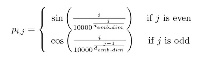
Value to be added to the i-th tensor in its j-th coordinate. Image source.
This positional embedding is a function of the number of elements in the sequence and the dimensionality of each element. Thus, it is always a 2-dimensional tensor or “rectangle”.
Here’s a simple function that, given the number of tokens and the dimensionality of each of them, outputs a matrix where each coordinate (i,j) is the value to be added to token i in dimension j.
1def get_positional_embeddings(sequence_length, d):
2    result = torch.ones(sequence_length, d)
3    for i in range(sequence_length):
4        for j in range(d):
5            result[i][j] = np.sin(i / (10000 ** (j / d))) if j % 2 == 0 else np.cos(i / (10000 ** ((j - 1) / d)))
6    return result
7
8if __name__ == "__main__":
9    import matplotlib.pyplot as plt
10
11    plt.imshow(get_positional_embeddings(100, 300), cmap="hot", interpolation="nearest")
12    plt.show()
13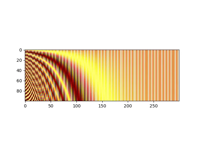
Heatmap of Positional embeddings for one hundred 300-dimensional samples. Samples are on the y-axis, whereas the dimensions are on the x-axis. Darker regions show higher values.
From the heatmap we have plotted, we see that all ‘horizontal lines’ are all different from each other, and thus samples can be distinguished.
We can now add this positional encoding to our model after the linear mapping and the addition of the class token.
1class MyViT(nn.Module):
2    def __init__(self, chw=(1, 28, 28), n_patches=7):
3        # Super constructor
4        super(MyViT, self).__init__()
5
6        # Attributes
7        self.chw = chw # (C, H, W)
8        self.n_patches = n_patches
9
10        assert chw[1] % n_patches == 0, "Input shape not entirely divisible by number of patches"
11        assert chw[2] % n_patches == 0, "Input shape not entirely divisible by number of patches"
12        self.patch_size = (chw[1] / n_patches, chw[2] / n_patches)
13
14        # 1) Linear mapper
15        self.input_d = int(chw[0] * self.patch_size[0] * self.patch_size[1])
16        self.linear_mapper = nn.Linear(self.input_d, self.hidden_d)
17
18        # 2) Learnable classifiation token
19        self.class_token = nn.Parameter(torch.rand(1, self.hidden_d))
20
21        # 3) Positional embedding
22        self.pos_embed = nn.Parameter(torch.tensor(get_positional_embeddings(self.n_patches ** 2 + 1, self.hidden_d)))
23        self.pos_embed.requires_grad = False
24
25    def forward(self, images):
26        patches = patchify(images, self.n_patches)
27        tokens = self.linear_mapper(patches)
28
29        # Adding classification token to the tokens
30        tokens = torch.stack([torch.vstack((self.class_token, tokens[i])) for i in range(len(tokens))])
31
32        # Adding positional embedding
33        pos_embed = self.pos_embed.repeat(n, 1, 1)
34        out = tokens + pos_embed
35        return out
36
We define the positional embedding to be a parameter of our model (that we won’t update by setting its requires_grad to False). Note that in the forward method, since tokens have size (N, 50, 8), we have to repeat the (50, 8) positional encoding matrix N times.
Step 4: The encoder block (Part 1/2)
This is possibly the hardest step of all. An encoder block takes as input our current tensor (N, S, D) and outputs a tensor of the same dimensionality.
The first part of the encoder block applies Layer Normalization to our tokens, then a Multi-head Self Attention, and finally adds a residual connection.
Layer Normalization
Layer normalization is a popular block that, given an input, subtracts its mean and divides by the standard deviation.
However, we commonly apply layer normalization to an (N, d) input, where d is the dimensionality. Luckily, also the Layer Normalization module generalizes to multiple dimensions, check this:
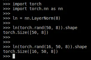
nn.LayerNorm can be applied in multiple dimensions. We can normalize fifty 8-dimensional vectors, but we can also normalize sixteen by fifty 8-dimensional vectors.
Layer normalization is applied to the last dimension only. We can thus make each of our 50x8 matrices (representing a single sequence) have mean 0 and std 1. After we run our (N, 50, 8) tensor through LN, we still get the same dimensionality.
Multi-Head Self-Attention
We now need to implement sub-figure c of the architecture picture. What’s happening there?
Simply put: we want, for a single image, each patch to get updated based on some similarity measure with the other patches. We do so by linearly mapping each patch (that is now an 8-dimensional vector in our example) to 3 distinct vectors: q, k, and v (query, key, value).
Then, for a single patch, we are going to compute the dot product between its q vector with all of the k vectors, divide by the square root of the dimensionality of these vectors (sqrt(8)), softmax these so-called attention cues, and finally multiply each attention cue with the v vectors associated with the different k vectors and sum all up.
In this way, each patch assumes a new value that is based on its similarity (after the linear mapping to q, k, and v) with other patches. This whole procedure, however, is carried out H times on H sub-vectors of our current 8-dimensional patches, where H is the number of Heads. If you’re unfamiliar with the attention and multi-head attention mechanisms, I suggest you read this nice post by Yasuto Tamura.
Once all results are obtained, they are concatenated together. Finally, the result is passed through a linear layer (for good measure).
The intuitive idea behind attention is that it allows modeling the relationship between the inputs. What makes a ‘0’ a zero are not the individual pixel values, but how they relate to each other.
Since quite some computations are carried out, it is worth creating a new class for MSA:
1class MyMSA(nn.Module):
2    def __init__(self, d, n_heads=2):
3        super(MyMSA, self).__init__()
4        self.d = d
5        self.n_heads = n_heads
6
7        assert d % n_heads == 0, f"Can't divide dimension {d} into {n_heads} heads"
8
9        d_head = int(d / n_heads)
10        self.q_mappings = nn.ModuleList([nn.Linear(d_head, d_head) for _ in range(self.n_heads)])
11        self.k_mappings = nn.ModuleList([nn.Linear(d_head, d_head) for _ in range(self.n_heads)])
12        self.v_mappings = nn.ModuleList([nn.Linear(d_head, d_head) for _ in range(self.n_heads)])
13        self.d_head = d_head
14        self.softmax = nn.Softmax(dim=-1)
15
16    def forward(self, sequences):
17        # Sequences has shape (N, seq_length, token_dim)
18        # We go into shape    (N, seq_length, n_heads, token_dim / n_heads)
19        # And come back to    (N, seq_length, item_dim)  (through concatenation)
20        result = []
21        for sequence in sequences:
22            seq_result = []
23            for head in range(self.n_heads):
24                q_mapping = self.q_mappings[head]
25                k_mapping = self.k_mappings[head]
26                v_mapping = self.v_mappings[head]
27
28                seq = sequence[:, head * self.d_head: (head + 1) * self.d_head]
29                q, k, v = q_mapping(seq), k_mapping(seq), v_mapping(seq)
30
31                attention = self.softmax(q @ k.T / (self.d_head ** 0.5))
32                seq_result.append(attention @ v)
33            result.append(torch.hstack(seq_result))
34        return torch.cat([torch.unsqueeze(r, dim=0) for r in result])
35
Notice that, for each head, we create distinct Q, K, and V mapping functions (square matrices of size 4x4 in our example).
Since our inputs will be sequences of size (N, 50, 8), and we only use 2 heads, we will at some point have an (N, 50, 2, 4) tensor, use a nn.Linear(4, 4) module on it, and then come back, after concatenation, to an (N, 50, 8) tensor.
Also notice that using loops is not the most efficient way to compute the multi-head self-attention, but it makes the code much clearer for learning.
Residual connection
A residual connection consists in just adding the original input to the result of some computation. This, intuitively, allows a network to become more powerful while also preserving the set of possible functions that the model can approximate.
We will add a residual connection that will add our original (N, 50, 8) tensor to the (N, 50, 8) obtained after LN and MSA. It’s time to create the transformer encoder block class, which will be a component of the MyViT class:
1class MyViTBlock(nn.Module):
2    def __init__(self, hidden_d, n_heads, mlp_ratio=4):
3        super(MyViTBlock, self).__init__()
4        self.hidden_d = hidden_d
5        self.n_heads = n_heads
6
7        self.norm1 = nn.LayerNorm(hidden_d)
8        self.mhsa = MyMSA(hidden_d, n_heads)
9
10    def forward(self, x):
11        out = x + self.mhsa(self.norm1(x))
12        return out
13
Phew, that was quite some work! But I promise this was the hardest part. From now on, it’s all downhill.
With this self-attention mechanism, the class token (first token of each of the N sequences) now has information regarding all other tokens!
Step 5: The encoder block (Part 2/2)
All that is left to the transformer encoder is just a simple residual connection between what we already have and what we get after passing the current tensor through another LN and an MLP. The MLP is composed of two layers, where the hidden layer typically is four times as big (this is a parameter)
1class MyViTBlock(nn.Module):
2    def __init__(self, hidden_d, n_heads, mlp_ratio=4):
3        super(MyViTBlock, self).__init__()
4        self.hidden_d = hidden_d
5        self.n_heads = n_heads
6
7        self.norm1 = nn.LayerNorm(hidden_d)
8        self.mhsa = MyMSA(hidden_d, n_heads)
9        self.norm2 = nn.LayerNorm(hidden_d)
10        self.mlp = nn.Sequential(
11            nn.Linear(hidden_d, mlp_ratio * hidden_d),
12            nn.GELU(),
13            nn.Linear(mlp_ratio * hidden_d, hidden_d)
14        )
15
16    def forward(self, x):
17        out = x + self.mhsa(self.norm1(x))
18        out = out + self.mlp(self.norm2(out))
19        return out
20
We can indeed see that the Encoder block outputs a tensor of the same dimensionality:
1if __name__ == '__main__':
2    model = MyVitBlock(hidden_d=8, n_heads=2)
3
4    x = torch.randn(7, 50, 8)  # Dummy sequences
5    print(model(x).shape)      # torch.Size([7, 50, 8])
6
Now that the encoder block is ready, we just need to insert it in our bigger ViT model which is responsible for patchifying before the transformer blocks, and carrying out the classification after.
We could have an arbitrary number of transformer blocks. In this example, to keep it simple, I will use only 2. We also add a parameter to know how many heads does each encoder block will use.
1class MyViT(nn.Module):
2    def __init__(self, chw, n_patches=7, n_blocks=2, hidden_d=8, n_heads=2, out_d=10):
3        # Super constructor
4        super(MyViT, self).__init__()
5
6        # Attributes
7        self.chw = chw # ( C , H , W )
8        self.n_patches = n_patches
9        self.n_blocks = n_blocks
10        self.n_heads = n_heads
11        self.hidden_d = hidden_d
12
13        # Input and patches sizes
14        assert chw[1] % n_patches == 0, "Input shape not entirely divisible by number of patches"
15        assert chw[2] % n_patches == 0, "Input shape not entirely divisible by number of patches"
16        self.patch_size = (chw[1] / n_patches, chw[2] / n_patches)
17
18        # 1) Linear mapper
19        self.input_d = int(chw[0] * self.patch_size[0] * self.patch_size[1])
20        self.linear_mapper = nn.Linear(self.input_d, self.hidden_d)
21
22        # 2) Learnable classification token
23        self.class_token = nn.Parameter(torch.rand(1, self.hidden_d))
24
25        # 3) Positional embedding
26        self.register_buffer('positional_embeddings', get_positional_embeddings(n_patches ** 2 + 1, hidden_d), persistent=False)
27
28        # 4) Transformer encoder blocks
29        self.blocks = nn.ModuleList([MyViTBlock(hidden_d, n_heads) for _ in range(n_blocks)])
30
31    def forward(self, images):
32        # Dividing images into patches
33        n, c, h, w = images.shape
34        patches = patchify(images, self.n_patches).to(self.positional_embeddings.device)
35
36        # Running linear layer tokenization
37        # Map the vector corresponding to each patch to the hidden size dimension
38        tokens = self.linear_mapper(patches)
39
40        # Adding classification token to the tokens
41        tokens = torch.cat((self.class_token.expand(n, 1, -1), tokens), dim=1)
42
43        # Adding positional embedding
44        out = tokens + self.positional_embeddings.repeat(n, 1, 1)
45
46        # Transformer Blocks
47        for block in self.blocks:
48            out = block(out)
49
50        return out
51
Once more, if we run a random (7, 1, 28, 28) tensor through our model, we still get a (7, 50, 8) tensor.
Step 6: Classification MLP
Finally, we can extract just the classification token (first token) out of our N sequences, and use each token to get N classifications.
Since we decided that each token is an 8-dimensional vector, and since we have 10 possible digits, we can implement the classification MLP as a simple 8x10 matrix, activated with the SoftMax function.
1class MyViT(nn.Module):
2    def __init__(self, chw, n_patches=7, n_blocks=2, hidden_d=8, n_heads=2, out_d=10):
3        # Super constructor
4        super(MyViT, self).__init__()
5
6        # Attributes
7        self.chw = chw # ( C , H , W )
8        self.n_patches = n_patches
9        self.n_blocks = n_blocks
10        self.n_heads = n_heads
11        self.hidden_d = hidden_d
12
13        # Input and patches sizes
14        assert chw[1] % n_patches == 0, "Input shape not entirely divisible by number of patches"
15        assert chw[2] % n_patches == 0, "Input shape not entirely divisible by number of patches"
16        self.patch_size = (chw[1] / n_patches, chw[2] / n_patches)
17
18        # 1) Linear mapper
19        self.input_d = int(chw[0] * self.patch_size[0] * self.patch_size[1])
20        self.linear_mapper = nn.Linear(self.input_d, self.hidden_d)
21
22        # 2) Learnable classification token
23        self.class_token = nn.Parameter(torch.rand(1, self.hidden_d))
24
25        # 3) Positional embedding
26        self.register_buffer('positional_embeddings', get_positional_embeddings(n_patches ** 2 + 1, hidden_d), persistent=False)
27
28        # 4) Transformer encoder blocks
29        self.blocks = nn.ModuleList([MyViTBlock(hidden_d, n_heads) for _ in range(n_blocks)])
30
31        # 5) Classification MLPk
32        self.mlp = nn.Sequential(
33            nn.Linear(self.hidden_d, out_d),
34            nn.Softmax(dim=-1)
35        )
36
37    def forward(self, images):
38        # Dividing images into patches
39        n, c, h, w = images.shape
40        patches = patchify(images, self.n_patches).to(self.positional_embeddings.device)
41
42        # Running linear layer tokenization
43        # Map the vector corresponding to each patch to the hidden size dimension
44        tokens = self.linear_mapper(patches)
45
46        # Adding classification token to the tokens
47        tokens = torch.cat((self.class_token.expand(n, 1, -1), tokens), dim=1)
48
49        # Adding positional embedding
50        out = tokens + self.positional_embeddings.repeat(n, 1, 1)
51
52        # Transformer Blocks
53        for block in self.blocks:
54            out = block(out)
55
56        # Getting the classification token only
57        out = out[:, 0]
58
59        return self.mlp(out) # Map to output dimension, output category distribution
60
The output of our model is now an (N, 10) tensor. Hurray, we are done!
Results
We change the only line in the main program that was previously undefined.
1model = MyVit((1, 28, 28), n_patches=7, n_blocks=2, hidden_d=8, n_heads=2, out_d=10).to(device)
2
We now just need to run the training and test loops and see how our model performs. If you’ve set torch seed manually (to 0), you should get this printed:
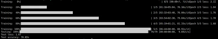
Training losses, test loss, and test accuracy obtained.
And that’s it! We have now created a ViT from scratch. Our model achieves ~80% accuracy in just 5 epochs and with few parameters.
You can find the full script at the following link. Let me know if this post was useful or think something was unclear!